Tutorial
Introduction
In this tutorial, you will learn how to upload dataset to the system and start a training environment (lab) in the system.
This tutorial uses Dog Breed Identification dataset to train a classification model to identify dog breeds.
Upload Dataset
First, click ‘New Dataset’ button in dataset page to create an empty directory.
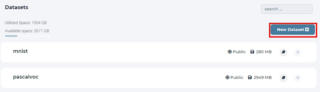
click New Dataset in dataset page.
Input the dataset name ‘Dog_Breed_Identification’.

name the dataset as ‘Dog_Breed_Identification’.
Download the Dog Breed Identification archive file to your PC.
In the previous created Dog_Breed_Identification dataset, click Add Dataset button to upload the archive dataset from you PC.
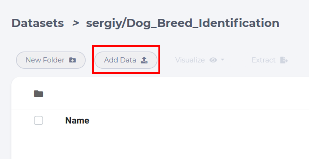
click upload button to select files
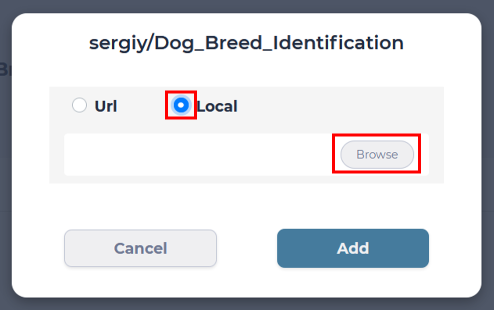
Tick Local to select files from your PC and then Browse
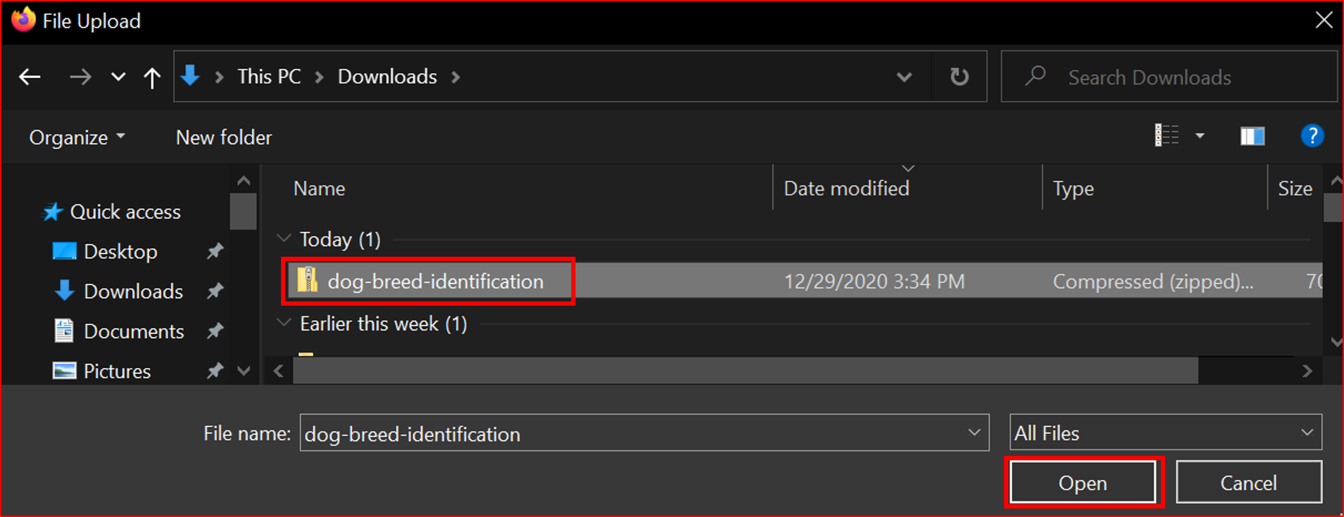
choose the archive file.
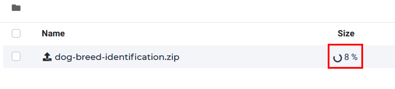
uploading.
After uploading done, choose the archive file and then click the Extract button. It takes a few seconds for extracting.
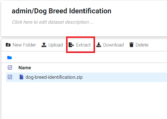
click extract button to extract the compressed file
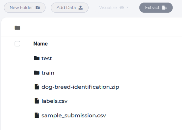
The file content should be same as shown below.
Create a LAB
Click LAB button in your project and click NEW LAB in Lab home page
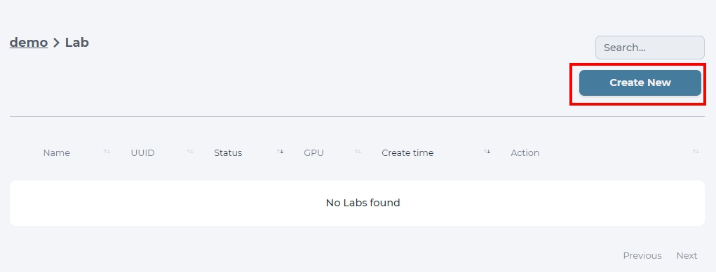
click NEW LAB to launch a modal.
Choose the python-gpu image and select “small” Flavor to support 1 GPU for this lab.
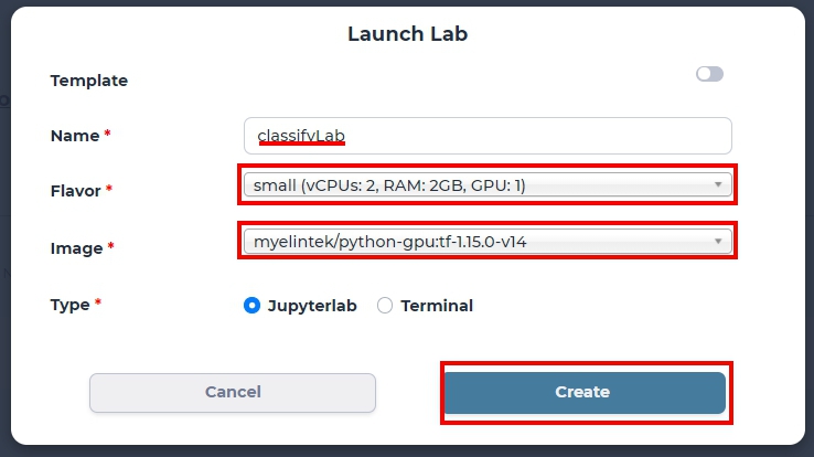
specify lab environment
Tip
If Flavor is set to micro, the created lab uses CPU only.
Attach Dataset to a LAB
Now we can attach the Dog Breed dataset to a LAB.
Open the Lab page, click the dataset icon at top-right of the Lab page. Select Dog Breed dataset.
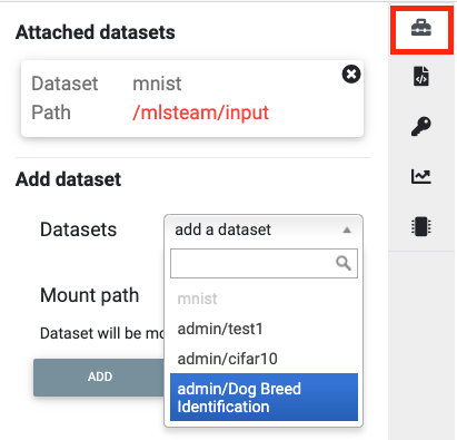
select dataset at top-right of the Lab page
Click Add button first, and then Attach Dataset button and confirm the warning, the LAB will restart for dataset connection.
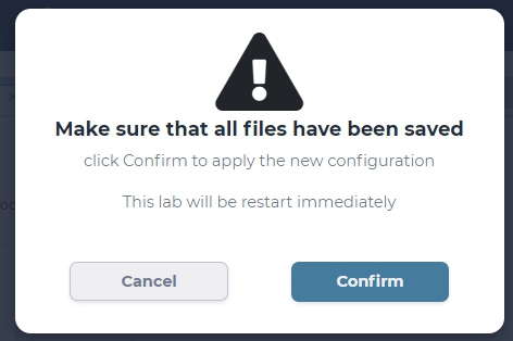
lab will restart for attaching selected dataset
Write a Notebook file for training
Start a notebook
Click the ‘+’ button if you can’t find the launcher tab.
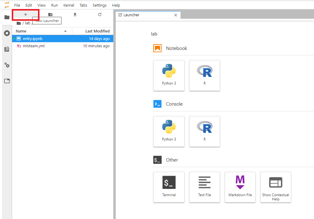
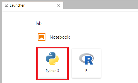
create a python3 notebook.
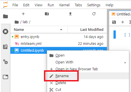
rename the notebook file to ‘dog_breed.ipynb’.
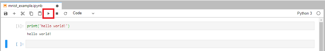
In the notebook, click ‘+’ to add a cell and click run button to executed the selected cell. Here is an example to execute the cell.
Dataset Preprocessing
The dog breed dataset contains different breeds of dogs images. The folder structure should be like this:
input -|
       |- test -
       |- train -
       |- labels.csv
       |- sample_submission.csv
The labels.csv records mappings of each dog image path and related label of breeds.
First, define path of data:
import os

base_folder = '/mlsteam/input'
train_folder = os.path.join(base_folder, 'train')
test_folder = os.path.join(base_folder, 'test')

label_file = os.path.join(base_folder, 'labels.csv')
The dataset contains 120 breeds, but we only select the most common 20 breeds for simplicity.
For verifying model accuracy during training, we take 20% of training images as validation dataset. The following code reads labels.csv and produce the train_df and valid_df, each contains a dataframe consists of many (id, breed) pairs.
import pandas as pd
import random

train_label = pd.read_csv(label_file)
NUM_CLASSES = 20

random.seed(NUM_CLASSES)

top_num_breed = list(train_label.groupby('breed').count().sort_values(by='id', ascending=False).head(NUM_CLASSES).index)

train_df = pd.DataFrame()
valid_df = pd.DataFrame()

ratio = 0.8
print('{:<20} {:>10} {:>10} {:>10}'.format('Breed', 'Total', 'Train', 'Valid'))
print('-'*60)
for breed in top_num_breed:
    tmp = train_label.loc[train_label['breed'].isin([breed])].reset_index(drop=True)
    train_num = int(len(tmp) * 0.8)
    print('{:<20} {:10} {:10} {:10}'.format(breed, len(tmp), train_num, len(tmp) - train_num))

    # random
    tmp_list = list(range(len(tmp)))
    random.shuffle(tmp_list)

    train_df = train_df.append(tmp.iloc[tmp_list[:train_num]], ignore_index=True)
    valid_df = valid_df.append(tmp.iloc[tmp_list[train_num:]], ignore_index=True)

for i, row in train_df.iterrows():
    train_df.at[i, 'id'] = row['id'] + '.jpg'

for i, row in valid_df.iterrows():
    valid_df.at[i, 'id'] = row['id'] + '.jpg'
Use ImageDataGenerator for model input
Create a image generator for training and add augmentation here, the parameters contains: the angle range of rotation, the shift range of horizontal and vertical direction, randomly flip images, and the switch of normalization for sample-wise.
from keras.preprocessing.image import ImageDataGenerator
train_datagen = ImageDataGenerator(
    #samplewise_center=True,
    #samplewise_std_normalization=True,
    rotation_range=45,
    width_shift_range=0.2,
    height_shift_range=0.2,
    shear_range=0.2,
    zoom_range=0.25,
    horizontal_flip=True,
    fill_mode='nearest',
    rescale=1./255
)
Then pass datafrme into a generator’s function, named flow_from_dataframe, this function get images name specified by ‘x_col’ and read image file as array type automaticlly.
train_generator = train_datagen.flow_from_dataframe(
                        dataframe=train_df,
                        directory=train_folder,
                        x_col="id",
                        y_col="breed",
                        class_mode="categorical",
                        target_size=(299, 299),
                        batch_size=32,
                        shuffle=True)
And we do the same thing for validation data, it’s worth to mention that we shouldn’t add any augmentation on valid data, except the rescale parameter.
valid_generator = ImageDataGenerator(rescale=1./255).flow_from_dataframe(
                        dataframe=valid_df,
                        directory=train_folder,
                        x_col="id",
                        y_col="breed",
                        class_mode="categorical",
                        target_size=(299, 299),
                        batch_size=32,
                        shuffle=False)
Model Training
We use the pre-trained Xception model and building new laypers on top for Transfer Learning.
### MODEL - BOTTLENECK FEATURES - OPTMIZER

from keras.layers import GlobalAveragePooling2D, Dense, BatchNormalization, Dropout
from keras.optimizers import Adam, SGD, RMSprop
from keras.models import Model, Input
from keras.applications import xception

# Download and create the pre-trained Xception model for transfer learning
base_model = xception.Xception(weights='imagenet', include_top=False)

# add a global spatial average pooling layer
x = base_model.output
x = BatchNormalization()(x)
x = GlobalAveragePooling2D()(x)
# let's add a fully-connected layer
x = Dropout(0.5)(x)
x = Dense(1024, activation='relu')(x)
x = Dropout(0.5)(x)
# and a logistic layer -- let's say we have NUM_CLASSES classes
predictions = Dense(NUM_CLASSES, activation='softmax')(x)

# this is the model we will train
model = Model(inputs=base_model.input, outputs=predictions)

# first: train only the top layers (which were randomly initialized)
# i.e. freeze all convolutional Xception layers
for layer in base_model.layers:
    layer.trainable = False

# compile the model (should be done *after* setting layers to non-trainable)
optimizer = RMSprop(lr=0.001, rho=0.9)
model.compile(optimizer=optimizer,
            loss='categorical_crossentropy',
            metrics=["accuracy"])
model.summary()
Start Training and validation for 10 epochs.
Training shows the progress bar of every epoch, the loss and accuracy will be printed behind each bar.
from keras.callbacks import TensorBoard, ModelCheckpoint, Callback

class TrainLogger(Callback):
    def on_epoch_begin(self, epoch, logs={}):
        self.epoch = epoch
    def on_train_batch_end(self, batch, logs={}):
        print("Train epoch={:.6f} loss={:.6f} acc={:.6f}".format(self.epoch+batch/self.params.get('steps'), logs.get('loss'), logs.get('accuracy')))
    def on_epoch_end(self, epoch, logs={}):
        print("Validation epoch={:.6f} loss={:.6f} acc={:.6f}".format(epoch+1.0, logs.get('val_loss'), logs.get('val_accuracy')))

tb_callBack = TensorBoard(log_dir='./tb', histogram_freq=0, write_graph=True, write_images=True)
model_checkpoint = ModelCheckpoint(filepath='./checkpoints', monitor='loss', verbose=0, save_best_only=True)

model.fit_generator(train_generator,
                    epochs=10,
                    steps_per_epoch=train_generator.n // train_generator.batch_size,
                    validation_data=valid_generator,
                    verbose=0,
                    callbacks=[tb_callBack, model_checkpoint, TrainLogger()])
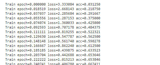
training output.
Tensorboard visualization
A Tensorboard can be launched from web, at right sidebar menu, speficy the logdir path for tensorboard to read the summary files.

input logdir path for tensorboard to read the summary files.
Click the url for starting TensorBoard.

After training finished, we can save the model parameters as a HDF5 format by following command.
model.save('my_model.h5')
Evaluate Model
We can evaluate the model by producing confusion matrix from validation images.
from sklearn.metrics import confusion_matrix
import numpy as np

valid_pred = model.predict_generator(valid_generator, verbose=1)
cnf_matrix = confusion_matrix(valid_generator.labels,  np.argmax(valid_pred,axis=1))
And plot the generated confusion matrix:
# Mapping
breed_mapping = {v: k for k, v in train_generator.class_indices.items()}

breed_list = [b for b in breed_mapping.values()]
df_cm = pd.DataFrame(cnf_matrix, index=breed_list, columns=breed_list)

import matplotlib.pyplot as plt

fig = plt.figure(figsize=(10, 7))
try:
    import seaborn as sns
    heatmap = sns.heatmap(df_cm, annot=True, fmt="d")
except ValueError:
    raise ValueError("Confusion matrix values must be integers.")

heatmap.yaxis.set_ticklabels(heatmap.yaxis.get_ticklabels(), rotation=0, ha='right', fontsize=10)
heatmap.xaxis.set_ticklabels(heatmap.xaxis.get_ticklabels(), rotation=45, ha='right', fontsize=10)
plt.title('Confusion Matrix')
plt.ylabel('True label')
plt.xlabel('Predicted label')

plt.show()
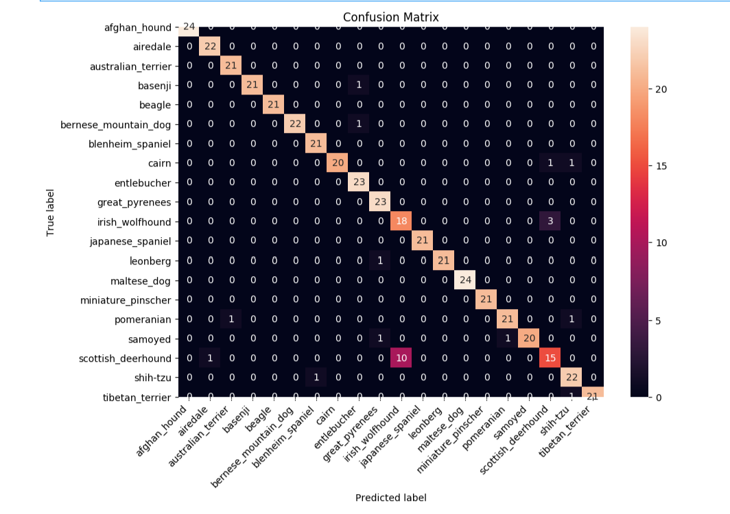
Image Prediction
The test_folder in the dataset contains 10360 images to be predicted.
Here we load the test images and create the test_generator for later prediction.
def get_imgs(path):
    imgs = []
    for entry in os.scandir(path):
        if entry.is_dir():
            imgs.extend(get_imgs(entry.path))
        else:
            imgs.append(entry.path)
    return imgs

test_imgs = get_imgs(test_folder)

test_df = pd.DataFrame({"x":test_imgs})

test_generator = ImageDataGenerator(rescale=1./255).flow_from_dataframe(
                        test_df,
                        x_col='x',
                        class_mode=None,
                        target_size=(299, 299),
                        batch_size=32,
                        shuffle=False)
We use the trained model to predict the test images:
pred = model.predict_generator(test_generator, verbose=1)
The prediction result is an array, it contains probability of breeds for each image.
Now, we need the mapping between index and breed name for readability.
breed_mapping = {v: k for k, v in train_generator.class_indices.items()}
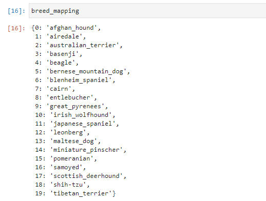
mapping between index and breed name
And, use the following code to display the test images with prediction results.
# Get first batch
test_generator.reset()
first_batch = test_generator.next()
(first_batch_imgs) = first_batch
first_batch_pred = pred[:len(first_batch_imgs)]

def get_max_index(array):
    max = 0
    max_index = 0
    for i in range(len(array)):
        if array[i] > max:
            max = array[i]
            max_index = i
    return max_index

# Mapping
breed_mapping = {v: k for k, v in train_generator.class_indices.items()}

# Start to Plot
import matplotlib.pyplot as plt

fig=plt.figure(figsize=(16, 16))
columns = 4
rows = 5

for i in range(1, columns*rows +1):
    fig.add_subplot(rows, columns, i)
    plt.tick_params(
        bottom=False,
        left=False,
        labelbottom=False,
        labelleft=False
    )
    plt.tight_layout(pad=2, h_pad=0.2, w_pad=0.2)
    plt.title(breed_mapping[get_max_index(first_batch_pred[i-1])])
    plt.imshow(first_batch_imgs[i-1])
plt.show()
plt.savefig('prediction_20.png')
The output should be like this:
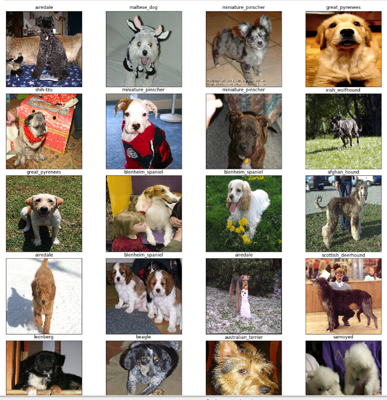
prediction results with trained model
Submit a training job
For advanced users who want to tune hyper-parameters, we suggest to run each training as a job for better organization.
You can download the above training code here file which includes above code.
Open mlsteam.yml in lab folder, specify the training job command ‘ipython3 dog_breed.ipynb’.
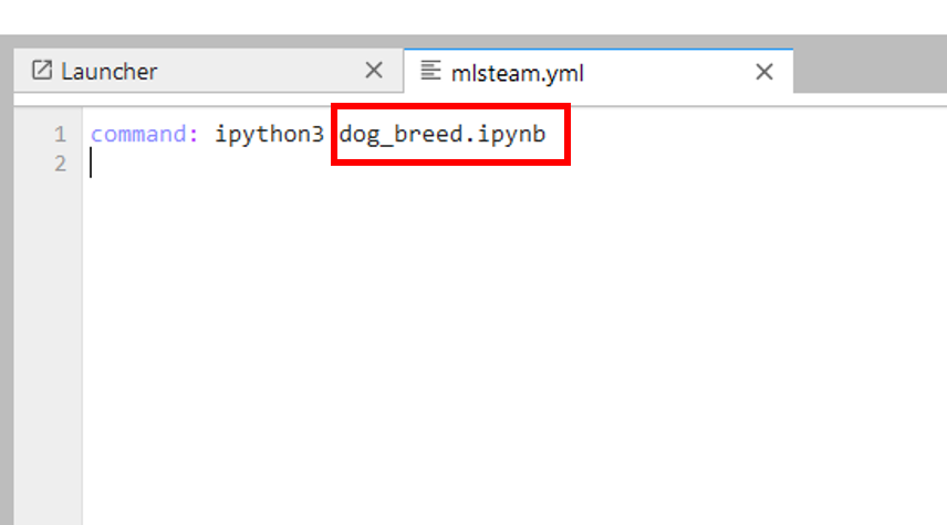
specify ‘command’ for training job
Click the ‘Submit Job’ button on top right of the lab and confirm the training parameters.
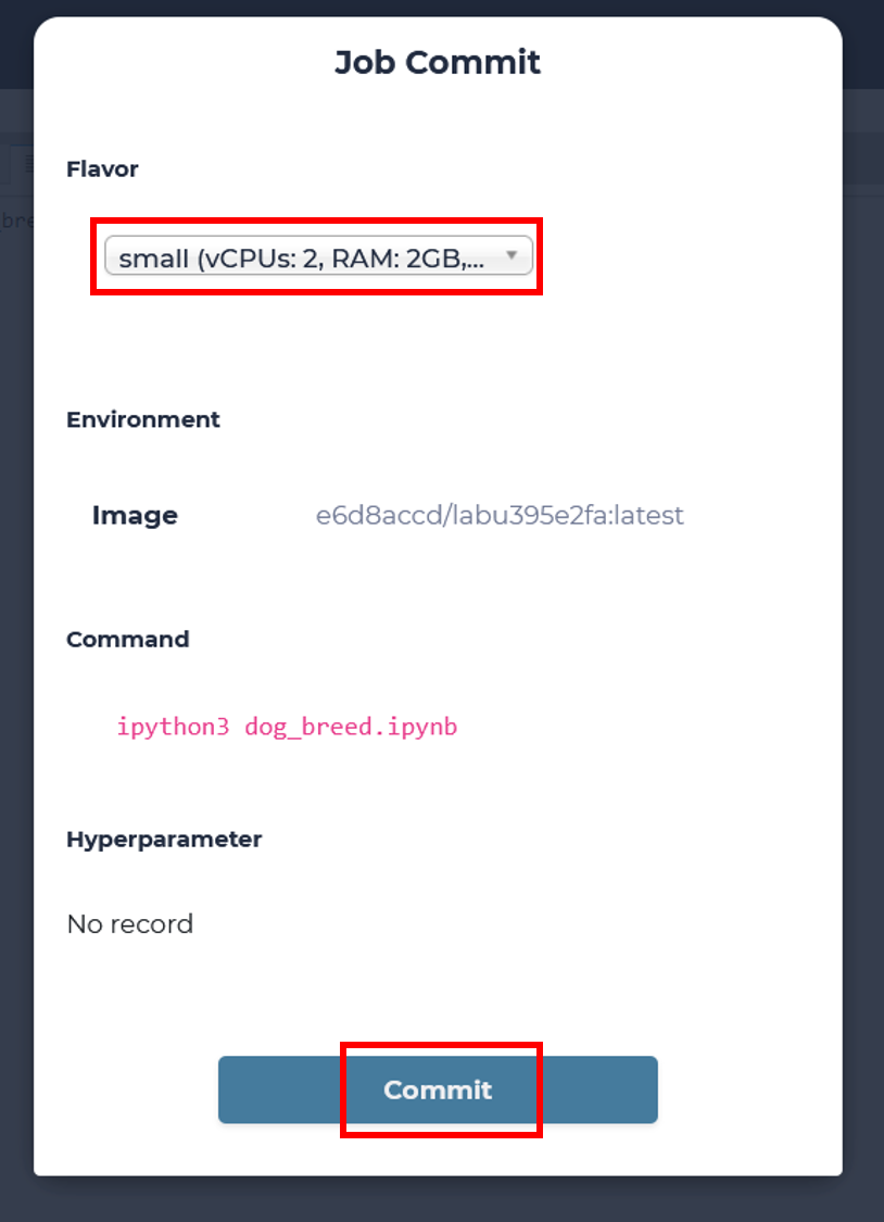
click commit to submit a training job
Note
choose a “small” flavor to use 1 GPU
You can click the new created training job for monitoring.
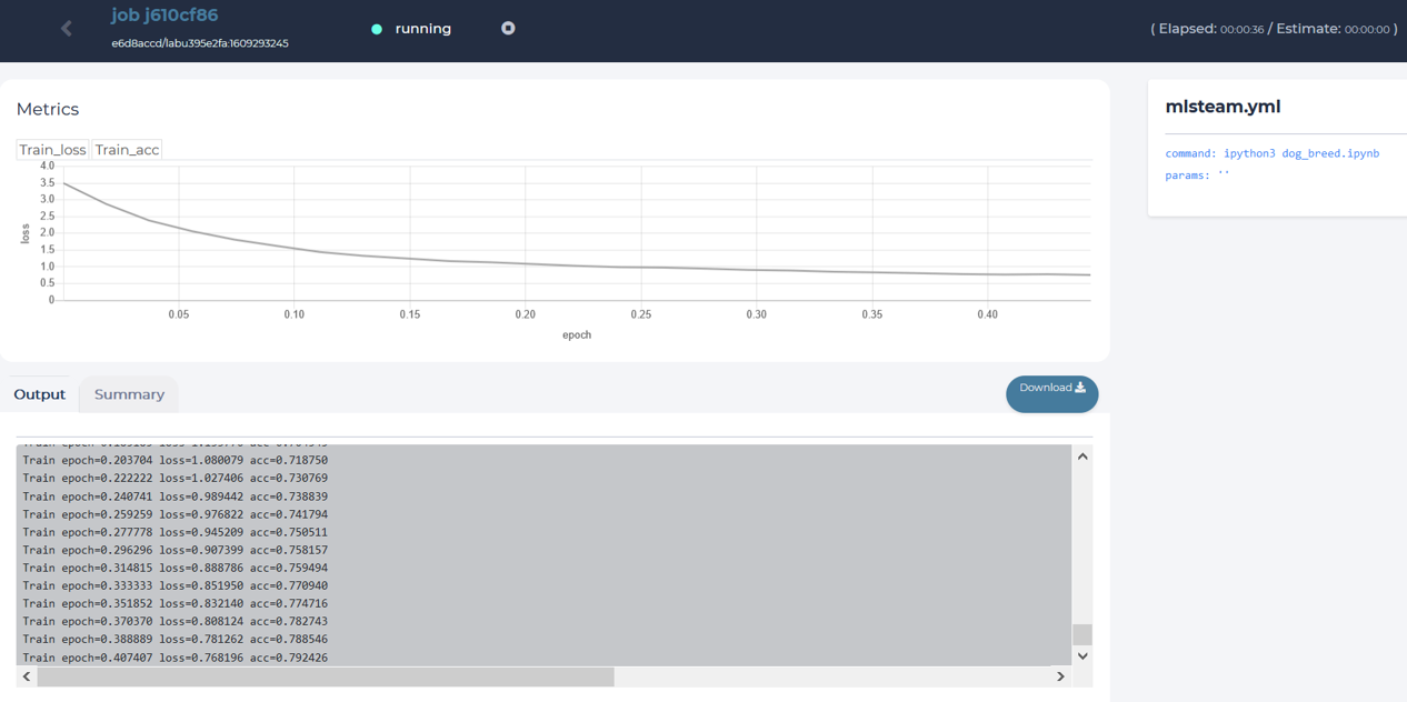
content of a training job page.